Parameter inference using Markov chain Monte Carlo algorithms and Haskell

We analyze the number of worldwide airline fatal accidents:

This table is an excerpt of Table 2.2 in Gelman, Andrew and Carlin, John B and Stern, Hal S and Rubin, Donald B (2014).

We assume that the number of fatal accidents \(X\) is Poisson distributed with fatal accident rate \(\lambda\)

\begin{align} Pr(X=k|\lambda) = \frac{\lambda^k e^{-\lambda}}{k!}. \end{align}

The maximum likelihood estimate of \(\lambda\) is the mean of the fatalities, which is \(23.8\). However, we infer the probability distribution of \(\lambda\) given the observed fatalities. Actually, we infer a function that is proportional to the probability distribution of \(\lambda\) but is not a distribution because it does not integrate to \(1.0\). We call this function posterior function.

We know that the true mode of the posterior function should be at \(\lambda = 23.8\), and so the mode of our estimate of the posterior function should be close. We use a Markov chain Monte Carlo (MCMC) sampler and Haskell.

Algorithm

Markov chains are sequences of events with a peculiar property: the probability of each possible next event only depends on the state of the previous event. In particular, the probability does not depend on any events before the previous event. Markov chains are widely used in statistics, for example, to predict the weather. An interesting application of Markov chains is MCMC, a class of algorithms used to effectively sample from probability distributions.

The answer is: Yes, and this is exactly what MCMC samplers do. For example, the most famous Metropolis-Hastings-Green algorithm (Geyer, Charles J, 2011, an excellent introduction to MCMC by the way) samples new values from given, well-behaved proposal distributions, only to accept or reject these new values according to the actual probability distribution of interest.

Note that standard probability distributions are heavily studied and there exist much faster, dedicated sampling methods. For example, see the computational methods to sample from the Poisson distribution or the normal distribution. Actually, the Metropolis-Hastings-Green algorithm makes use of these dedicated methods.

Implementation

In the following, we will implement the sampler using the mcmc library which I am developing. Here, I only briefly present the essential steps to run an MCMC sampler; please have a look at the documentation on Hackage, if you want to get a deeper understanding of the internals. Further, we use the random library, as well as the following imports:

-- We need 'void'.
import Control.Monad
-- I am developing the 'mcmc' library.
import Mcmc
-- We need to sample random numbers; requires the 'random' library.
import System.Random

The state space \(I\) of an MCMC sampler defines the possible values the Markov chain can attain. In our case \(I\) is the fatal accident rate \(\lambda\), a floating point number:

type I = Double

For a given fatal accident rate \(\lambda\), the likelihood function is a product of Poisson probabilities with the observed fatalities:

lh :: LikelihoodFunction I
lh x = product [poisson x y | y <- fatalities]
  where
    fatalities = [24, 25, 31, 31, 22, 21, 26, 20, 16, 22]

The LikehoodFunction I is a type synonym for I -> Log Double. Internally, we use probabilities in the log domain to avoid numerical underflow; see log-domain.

We need to tell the sampler how to propose new values. We do this using proposals. Here, we use two types:

• a sliding proposal which adds random numbers to the current value of \(\lambda\), and
• a scaling proposal which multiplies random values with the current value of \(\lambda\).

ppSl :: Proposal I
ppSl = slideSymmetric 0.1 (PName "lambda") (pWeight 1) Tune

ppSc :: Proposal I
ppSc = scaleUnbiased 0.1 (PName "lambda") (pWeight 1) Tune

There is some necessary boiler plate code about how large the proposal sizes are, how we name the proposals, or what weight we assign to the proposals. Tune tells the MCMC sampler to tune the proposal size according to established optimization criteria. In particular, the acceptance rates of proposals have optimal values that depend on the proposal dimension. The proposal dimension roughly corresponds to the number of independent parameters manipulated by the proposal. Tuning only happens during the first phase of the sampler which is called burn in (more about that below).

We collect the proposals in a cycle:

cc :: Cycle I
cc = cycleFromList [ppSl, ppSc]

This modular definition of proposals, that is, of how to traverse the state space is one of the big strengths of the mcmc library. For complicated state spaces, we can use liftProposal and lenses to inform proposals about what part of the state they should change.

Now, we define some monitors, so that we can observe the values of \(\lambda\) attained by the Markov chain:

-- 'monitorDouble' is a simple monitor printing the value of a 'Double'.
monLambda :: MonitorParameter I
monLambda = monitorDouble "lambda"

-- We print the value of lambda to the standard output every 100 iterations.
monStdOut :: MonitorStdOut I
monStdOut = monitorStdOut [monLambda] 100

-- We log the value of lambda to a file more often.
monFile :: MonitorFile I
monFile = monitorFile "lambda" [monLambda] 3

mon :: Monitor I
mon = Monitor monStdOut [monFile] []

We do not use batch monitors, so the last list of mon is empty.

Before running the chain, we need to provide some required settings:

ss :: Settings
ss =
  Settings
    -- Provide an analysis name.
    (AnalysisName "poisson")
    -- Burn in for 2000 generations. During burn in, the proposals are tuned
    -- automatically. This is called "auto tuning". Here, auto tuning is
    -- performed every 200 iterations.
    (BurnInWithAutoTuning 2000 200)
    -- Number of actual iterations after burn in.
    (Iterations 30000)
    -- The trace of the Markov chain contains the attained values. In our case,
    -- it is a vector of fatal accident rates. Here, we tell the sampler to use
    -- the shortest trace possible. In our case, this will be a single value.
    -- However, when using batch monitors, or when auto tuning the masses of
    -- proposals based on Hamiltonian dynamics, the required length of the trace
    -- is larger than 1. masses. The trace length can also be set manually.
    TraceAuto
    -- Overwrite files created by a possible previous analysis.
    Overwrite
    -- Do not run chains in parallel. For the standard Metropolis-Hastings-Green
    -- algorithm, this has no effect. However, there are algorithms such as the
    -- MC3 algorithm with multiple chains that can run in parallel.
    Sequential
    -- Save the chain so that it can be continued (see 'mcmcContinue').
    Save
    -- Log to standard output and save the log to a file.
    LogStdOutAndFile
    -- Verbosity.
    Info

Finally, we instantiate a chain using the Metropolis-Hastings-Green algorithm (MHG, mhg function) and run the MCMC sampler with the mcmc function:

main :: IO ()
main = do
  let g = mkStdGen 0
  -- Set up the Markov chain. For computational efficiency (mutable vectors),
  -- this requires IO.
  al <- mhg ss noPrior lh cc mon 1.0 g
  -- We ignore the actual return value which is the complete Markov chain object
  -- using 'void'.
  void $ mcmc ss al

The complete code is available in the mcmc Git repository, see also the accompanying Cabal file.

Results

Using the above mentioned Git repository, you can run the code with

cabal run poisson

There is a lot of informative output. Further, log files poisson.mcmc.* and the monitor file poisson.lambda.monitor are created. Here, I will have a look at the posterior function of \(\lambda\). To this end, I use Tracer to inspect the monitor file poisson.lambda.monitor:

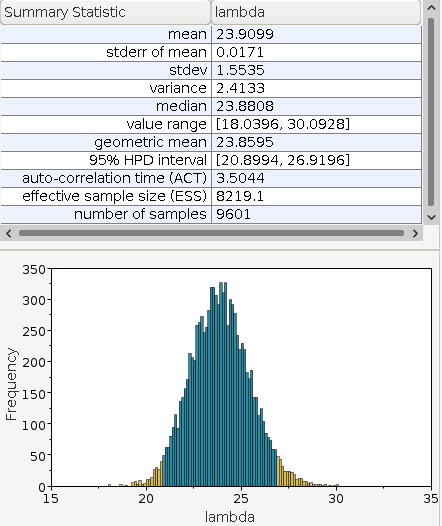
We see in the summary statistics, that the estimated median is \(23.88\) which is close to the theoretical optimum of \(23.8\). We also observe that the posterior function is somewhat normal distributed.

Summary and outlook

We inferred the posterior function of the fatal accident rate of airlines in the 70s and 80s using a simple Poisson distribution, and an MCMC sampler in Haskell. There is a lot more we could do here. For example, we could improve our model using Poisson regression, we could look at advanced proposals such as proposals using Hamiltonian dynamics, or we could look at algorithms using parallel chains such as the Metropolic coupled MCMC (MC3) algorithm.

If this post spurred your interest, and you want to have a look at a real-life project: We use the mcmc library to perform phylogenetic dating. With McmcDate we infer the ages of speciations using molecular sequence data (DNA), molecular clocks, the age of fossils, gene transfers and much more! For example, we apply McmcDate to data from land plants (Harris, Brogan J. and Clark, James W. and Schrempf, Dominik and Szöllősi, Gergely J. and Donoghue, Philip C.J. and Hetherington, Alistair M. and Williams, Tom A., 2021).

The mcmc library is under development, and I am happy about your suggestions or comments; drop them on the repository on GitHub!

References

Gelman, Andrew and Carlin, John B and Stern, Hal S and Rubin, Donald B (2014). Bayesian data analysis, CRC Press.

Geyer, Charles J (2011). {Introduction to Markov Chain Monte Carlo}, CRC press.

Harris, Brogan J. and Clark, James W. and Schrempf, Dominik and Szöllősi, Gergely J. and Donoghue, Philip C.J. and Hetherington, Alistair M. and Williams, Tom A. (2021). Divergent evolutionary trajectories of bryophytes and tracheophytes from a complex common ancestor of land plants.